Uncategorized | Big Numbers

Going to be out of commission January 11, 2011

Posted by Sarah in Uncategorized.
1 comment so far

I’m going to have to focus completely on school for a while so this blog is going on hiatus for a few months. I’ll start up again when I’ve passed the hurdles coming my way.

All done December 17, 2010

Posted by Sarah in Uncategorized.
add a comment

I’m finished with finals at last. Who knows how they’ll come out, but it’s a relief to be done at the moment. I’m finally getting my room clean, my laundry done, my presents bought, and my social life reanimated. And I’m looking at an introductory (very introductory) AI textbook here.

Also, for those looking for a non-corny holiday movie, I recommend seeing Holiday while it’s still on Hulu. Cary Grant, Katherine Hepburn, and a surprisingly modern story about following your own path.

NASA Finds New Life December 2, 2010

Posted by Sarah in Uncategorized.
add a comment

Stop what you’re doing, right now, and check this out.

NASA scientist Felisa Wolfe Simon has discovered a microbe with a different molecular structure than all life on Earth. While our molecules are made of carbon, hydrogen, oxygen, nitrogen, sulfur, and phosphorus, these single-celled organisms use arsenic in place of phosphorus. Its DNA is different from the DNA of all other life. This is the most alien creature we know.

The official announcement and live video is here.

Multiscale SVD, K planes and geometric wavelets November 30, 2010

Posted by Sarah in Uncategorized.
Tags: dimensionality reduction, geometric wavelets, high dimensional data, mauro maggioni, multiscale methods
add a comment

I went to the applied math talk by Mauro Maggioni today; here are notes from the presentation.

Multiscale SVD

We often have to deal with high-dimensional data clouds that may lie on a low-dimensional manifold. Examples: databases of faces, collections of text documents, configurations of molecules. But, we don’t know a priori what the dimension of the manifold is. So we ned some mechanisms for estimating that, in the situation where we have noise in the data.

Some terminology: the data points are $x_i + \eta_i$ , the real data plus some white Gaussian noise of variance $\sigma^2$ . The intrinsic dimension of the manifold $M$ is $k$ while the dimension of the ambient space is $D$ .

Previous work at estimating dimensions generally falls into two categories. One is volume-based (the number of points on the manifold confined within a ball should grow as $r^k$ where $r$ is the radius, if you’ve chosen the right dimension k. The other possibility is PCA, done locally and patched together somehow to account for the fact that we have a curved manifold rather than a linear hyperplane. The problem with this is that you don’t know what “locally” means — how many patches do we need? There’s also the so-called “curvature dilemma” with PCA: the more highly curved the manifold, the more likely it is to confuse the top principal value (representing the tangent direction) with the second-highest principal value (representing the direction of curvature.)

Maggioni’s alternative is multiscale SVD. We fix a point. The noise around the manifold looks like a hollow tube — most of the noise is concentrated at a radius of $\sigma \sqrt{D}$ from the surface of the manifold itself. So looking at a small ball (smaller than the radius of the tube) picks up less noise, looking at a large ball picks up all the noise, and looking at a still larger ball begins to pick up the curvature of the manifold. We do SVD within all these balls, and look at the singular values over a range of scales. There’s a “sweet spot,” a particular interval of scales where the signal singular values have separated from the noise singular values, but the curvature singular values haven’t caught up yet; this accurately represents the curvature of the manifold. (I blogged about this earlier here and the paper is here.)

The assumption about the data is that the tangent covariance grows differently ( $O(r^2)$ ) with respect to the radius than the normal covariance ( $O(r^4)$ ). This can be computed to be true explicitly for manifolds of co-dimension one, for instance.

The result is that if $M$ is assumed to have small enough curvature and $\eta$ is assumed to have small enough variance, then with high probability we can determine the intrinsic dimension $k$ with only $k \log k$ points. Compared to a large number of other dimension-estimating methods, this outperforms all of them. Isomap, in particular, really falls apart in the presence of noise, and can’t tell a 6-dimensional sphere from a 6-dimensional cube.

One interesting fact is that many real-life data sets have dimensionality that varies. A database of text documents, for instance, is low-dimensional in some regions, and very, very high-dimensional in others. (We measure dimensionality locally, so there’s no reason in principle that it shouldn’t vary.)

Measures supported on K planes
Sometimes high-dimensional data is supported on a set of planes $\pi_1 \dots \pi_k$ , possibly of different dimensions $d_1 \dots d_k$ . We don’t know how many planes there are, which planes they are, or what their dimensions are. This is the situation in face recognition; it’s also relevant to image and signal processing more generally (dictionary learning, sparse approximation, etc.)

Maggioni and collaborators developed an algorithm for doing this.

1) Draw $n_0$ random points and $n n_0$ nearest neighbors. Do multiscale SVD at these points. Produce an estimated plane $\hat{\pi}_k$ and its estimated dimension $\hat{d}_k$ . Also estimate the noise level $\hat{\sigma}$ .

2. Construct an affinity matrix, with the (i, j)th coordinate

$e^{\frac{-d(x_i, \hat{\pi}_k)^2}{\hat{\sigma}^2}}$

This is almost a matrix composed of zeros and ones — either a point is on a plane (in which we get one) or a point is not on that plane (in which case we get 0 because the distance is large.) In practice, with noise and curvature, it’s not quite binary, but it’s close.

3. Denoise and cluster this matrix, and find updated estimates for the planes from this.

Tested on a face database, this worked very well. It misclassified only 3 faces out of 640. What’s remarkable here is that the Yale Face Database used had 64 different photos of each person, taken at different angles, different lighting conditions, etc. This has always been a hard problem for computer vision: how do you recognize that two pictures are the same person viewed frontal and profile, while two other pictures are of two different people? Apparently, this is a solution to such heterogeneity problems.

Geometric wavelets
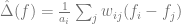
The problem of dictionary learning is as follows. Given $n$ points in $\mathbb{R}^D$ , and a data matrix $X$ , construct a dictionary $\Phi$ of m vectors such that

$X = \Phi \alpha$
where $\alpha$ is a sparse vector.

There’s a tradeoff here between the size of $\Phi$ and the sparsity of $\alpha$ : obviously, you could just let $\Phi$ be the whole of $X$ and then $\alpha$ would just be the identity, but that would be silly — it wouldn’t compress the data at all.

One way of doing this is something called geometric wavelets. (Paper here. Shorter, more descriptive paper with cool picture here.)
Given a manifold, we partition it into a dyadic tree. We do principal components analysis on the coarsest scale and get a plane; then we divide that into two smaller subsets, do PCA on each of them, and get two new planes. For each plane, at the center point of that cube in the manifold grid, we have a tangent vector $\Phi_j$ , which approximates the tangent to the manifold. The wavelets keep track of the differences $\Phi_j - \Phi_{j+1}$ . If we have some smoothness in the manifold, these corrections decay quickly, so finitely many wavelets are a good approximator for any point.

There’s a fast algorithm for computing this, very like the wavelet transform, except for a point cloud rather than a function. This is useful for compressing databases, analyzing online data, and so forth.

The idea is very like Peter Jones’ construction of beta numbers (summary here) except that it may be more efficient in terms of storage. More on geometric wavelets from Dan Lemire.

Vision without categories? November 17, 2010

Posted by Sarah in Uncategorized.
Tags: AI, computer vision, machine learning
add a comment

I’d just like to mention that I’ve come across Tomasz Malisiewicz’s blog on machine learning and computer vision, and I’m hooked. You should be too.

There’s the usual panoply of links to interesting papers, but then there’s also Tomasz’s radical idea for reimagining computer vision using a memex instead of a set of categories. He thinks that the “vision problem” will be solved by something much closer to actual AI than is generally considered necessary today. His ideas are informed by Wittgenstein and Vannevar Bush as well as contemporary research. It sounds interesting, to say the least. Then there’s also Tomasz’s stirring (if somewhat intimidating) advice to students and researchers to be Renaissance men and look beyond the A+ and the well-received publication. All in all, very worth reading.

(Sensible Sarah says: “Hey, wait a minute! I thought I was a math student — what’s up with all this vision stuff? And I have a qual to pass in a month!” Sensible Sarah throws up her hands in dismay.)

The Custom Essay Man November 16, 2010

Posted by Sarah in Uncategorized.
Tags: academia
3 comments

I was somewhat disturbed to read this article in the Chronicle of Higher Education. It’s written by a man who writes papers for a custom-essay company; students pay him to write their papers for them. Obviously it’s sad to see how common academic dishonesty is. But what really shocked me was something else.

A lot of “Ed Dante”‘s customers (he goes by a pseudonym) are in graduate or professional school. And apparently they’re really terrible writers. When they write him asking him for help, it’s something like “You did me business ethics propsal for me I need propsal got approved pls can you will write me paper?” I have to wonder — why are these people in graduate school in the first place?

I don’t mean that pejoratively. I don’t think you’re inferior as a person if you’re bad at writing or not gifted at academics. But look. I’m a grad student myself. I’m here because I want to be a mathematician. While the future is uncertain for all of us, I wouldn’t be here if I thought that was a completely unrealistic goal. If I were so overwhelmed by the work here that I was tempted to pay someone to do it for me, and if I’d already tried tutors, adjusting my sleep and study schedule, etc. then I’d start reevaluating my plans. It would be insane not to! The way I see it, going to graduate school is a decision that has to be justified — you should do it only if you think it’ll help you in the long run.

If you can’t write your own briefs in law school, you really think you’re going to be a successful lawyer? If you can’t write your own PhD thesis, do you really think you have any chance to make it in academia?

This article really makes me worry that lots of people are going for extra degrees just for the sake of doing it, or to escape the job market, and not because they’re really pursuing a passion or talent that has a realistic chance of paying off. That’s disturbing — it seems like a bad sign for the economy as a whole.

Shape Google November 15, 2010

Posted by Sarah in Uncategorized.
Tags: content-based image retrieval, image processing, laplace-beltrami operator, machine learning
2 comments

Currently reading this paper by Alex Bronstein et al.

The idea here is to make searchable databases for shapes (2d and 3d objects) in the same way a text engine responds to search queries.

There are two main parts to this task: feature detection, and feature description. Different methods can be employed to define what a feature is; a dense descriptor just selects all the points in the image as descriptors, but there are other possibilities. SIFT looks for local maxima of the discrete image Laplacian that persist through different scales. MSER finds level sets that show the smallest variation of area when traversing the level-set graph.

Feature description aims to produce a “bag of words” from the features, by performing vector quantization on the feature space. Two images can then be compared by comparing their bags of features with plain old Euclidean distance.

There are extra challenges if we want to do this with 3d objects rather than images: for one, conformations of 3d objects (like a body in different poses) are much more complicated than the (usually affine) transformations seen on a given image. Also, while images are typically represented as matrices of pixels, 3d objects can be represented as meshes, point clouds, level sets, etc, so computations have to be portable between formats. Also, 3d objects don’t have a universal system of coordinates.

The feature description process used by the authors is based on heat kernel signatures.
Recall that the heat kernel $K_t(x, z)$ is the fundamental solution of the heat equation
$(\Delta_x + \frac{\partial }{\partial t} )u = 0.$
The heat kernel can also be seen as the transition density function of a Brownian motion.
For any point on the surface, we give its heat kernel signature as
$p(x) = c(x)(K_{t_1}(x, x), K_{t_2}(x, x), \dots K_{t_n}(x, x))$
This is invariant under isometric deformations of the space, since it depends only on the Riemannian metric. It captures local information in a small neighborhood of x for small t, and global information for large t. It can be proven that any continuous map preserving the heat kernel signature must be an isometry. And computing it depends on computing the eigenvalues of the Laplacian, which can be done with various formats of representing 3d shapes.

$K_t(x, x') = \sum_{l = 0}^\infty e^{-\lambda_i t} \phi_l(x) \phi_l(x')$

So, since the eigenvalues of the Laplacian decay exponentially, we can truncate this sum for computation of the heat kernel.
In the discrete case, instead of the Laplacian we would use a discretization of the form

$\hat{\Delta} (f) = \frac{1}{a_i} \sum_j w_{ij} (f_i - f_j)$

After vector quantization to get a bag of features, the authors generalize this notion to a spatiall sensitive bag of features:

$\int_{X \times X} \theta(x) \theta^T(y) K_t(x, y) d\mu(x) d\mu(y)$
giving a matrix that represents the distribution of nearby words.

From there, we can compare these matrices by embedding them into a Hamming Space. (Hamming distances happen to be very quick to compute on modern CPU architectures.

ShapeGoogle was tested against various possible transformations of shapes (isometries, topology changes, holes, noise, scale changes) and performed well, outperforming other methods like Shape DNA, part-based bag of words, and clock matching bag of features.

It’s an interesting project, and I suspect that the ability to search shape databases will prove useful. Here’s a list of current content-based image retrieval search engines: both Google and Bing use these methods (as opposed to only looking at metadata.)

Alternating methods for SVD November 9, 2010

Posted by Sarah in Uncategorized.
Tags: dimensionality reduction, pca, random matrix theory
1 comment so far

Last week’s applied math seminar was Arthur Szlam, talking about alternating methods for SVD. I’m putting up some notes here; several results are presented without proof.

Given an m x n matrix A, we want to find the best rank k approximation to A.
There is an explicit solution to this problem, known as the singular value decomposition. We write
$A = U \Sigma V^T$
where $\Sigma$ is diagonal, $U, V$ are orthogonal. The columns of $U$ are the eigenvectors of $A^T A$ and the columns of $V$ are the eigenvectors of $A A^T$ . This costs $O(m^2 n)$ operations, and it’s a completely explicit solution. To get a rank-k approximation, we take
$\hat{U} \hat{\Sigma} \hat{V}^T$
where the “hat” means taking the first k columns of each matrix.
This is the best rank-k approximation, both in the sense of Frobenius norm and operator norm.

However, if $k << m$ , $O(m^2 n)$ time is wasteful. There are recent attempts to do this faster, in $O(mkn)$ time.

We fix k, and a small oversampling parameter p, and let $l = k + p$ . Draw an $l \times m$ random Gaussian matrix $\Omega$ , and set $Q^T = \Omega A$ .
Calculate the SVD, $\tilde{U} \tilde{\Sigma} \tilde{V}^T = Q$ , and set $U$ to be the first k columns of $\tilde{U}$ , etc.

Why does this work?

Well, pretend A is really of rank 5, for instance. Hit A with a random matrix. It is unlikely that any vector will be in the kernel of A. Whatever's left is in the range. So we're very likely to have the full range of A; we probably preserve the SVD. However, in real life we don't have a known rank k matrix.

What we have is a guarantee of quality, in terms of the decay of the singular values:
$E ||A - A Q Q^T|| \le [ 1 + \sqrt{\frac{k}{p-1}} + \frac{e \sqrt{k + p}}{p} \sqrt{m-k}] \sigma_{k +1}$

Here the expected value is taken over the random Gaussian draw, the norm is the operator norm, and $\sigma_{k + 1}$ is the k + 1th singular value; if A is really rank k, this is zero, and the expected error is therefore zero. If $\sigma_{k+1}$ is small, then the bound is good. We're in danger if m is large and $\sigma_{k+1}$ is not super small.

This actually happens, unfortunately. For example, in term document matrices, where a collection of text documents form the rows, and words form the columns, with a word count in each matrix entry indicating how often a word was used in each document. (A little imagination should indicate the importance of these kinds of matrices for semantic analysis.) These matrices are sparse and large, but their singular values decay slowly. So what can we do here?

We hit $\Omega$ by some more powers of A, to drive down the smaller eigenvalues. In practice, 10 or 15 times.
$Q_q^T = \Omega A (A^TA)^q$
Now we have a new estimate, depending on the power q.

$E ||A - A Q_q Q_q^T|| \le [1 + \sqrt{\frac{k}{p-1}} + \frac{p \sqrt{k + p}}{p} \sqrt{m-k}]^{1/2q + 1} \sigma_{k+1}$

This works, but it can be memory intensive to save all the intermediate powers. This is where the "alternating" method comes in.

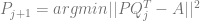
Here we look at a related problem: matrix completion. You're given a subset of the entries of a matrix A, and you know A is low rank. How do you fill in the rest of the entries? The simplest approach is alternating least squares.

Write $A = PQ^T$ where P is m-by-k and Q is n-by-k.
Alternate between updates of P and Q:
$P_{j+1} = argmin ||PQ_j^T - A||^2$
$Q_{j+1} = argmin ||P_{j-1} Q^T - A||$
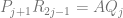
These are least-squares problems, and can be solved explicitly using

Step 1: form $m \times l$ Gaussian, $P_0$ .
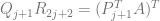
Step 2: form $n \times l$ matrix $Q_0$ st
$Q_0 R_0 = (P_0^T A)^T$
(a QR-decomposition, with Q orthogonal and R upper triangular.)
Step 3: iterate for $j = 0 \dots j = q-1$
$P_{j+1} R_{2j - 1} = A Q_j$
$Q_{j + 1} R_{2j +2} = (P_{j+1}^T A)^T$

Coming back to our own problem, we can use the same formula to calculate $Q_q^T$ .
$Q_j = (A^T A)^j A^T P_o (\prod_{s = 0}^{2j} R_s^{-1}.$

This turns out to work well in practice; the example set was a database of labeled faces, which have the first 20 eigenvalues decaying fast, then the next decaying very slowly. This kind of alternating SVD works well for faces.

Remember, Remember the Fifth of November November 5, 2010

Posted by Sarah in Uncategorized.
Tags: algebraic geometry
2 comments

Guy Fawkes Day. It’s a good day for radical ideals. No, not that kind! This kind.

I’m currently reading Charles Siegel’s series of posts on Algebraic Geometry from the beginning and I highly recommend. It’s some of the clearest, loveliest writing ever, and it’s got me really interested in the topic.

Advice for calculus students November 3, 2010

Posted by Sarah in Uncategorized.
Tags: grad life, teaching
5 comments

I am now a TA holding office hours for some calculus classes, and I actually enjoy it a lot. I’m generally impressed with the students. General advice that ought to hold if you’re taking an intro calc class:

1. Don’t freak out because a problem is taking a long time and seems unfairly hard. You’ll say “There must be some mistake!” No, there isn’t. This isn’t high school; you’re being taught by professors, who don’t always know how to gauge the right difficulty level. They do tend to underestimate how long it takes to finish your homework. Also, calculus is actually harder than high school math. If you have to go through a lot of computations and false steps — don’t worry! That’s what math is actually like!

2. I do not have magical TA superpowers of Mathematica. Most of the time, if you ask me for help, I’m going to look at the example on your worksheet and look in the help documentation. You could do that too! The xkcd Tech Support Cheat Sheet is relevant here.

3. L’Hopital’s rule is your friend. Seriously. So is big-O notation. These will save your bacon.

4. 90% of mistakes in multivariable calc result from not drawing pictures. Draw a picture. You are never too cool to draw a picture.

« older posts

Big Numbers